Student acceptance
Lately I got to play with some very interesting data, relating to student acceptance (and ranking) into applied courses from a university in Korea. The university (which name must be hidden) is a highly ranked university in Korea, and life there is super competetive in almost every way. It is therefore very interesting to see what drives acceptance, and what can students do to improve their chances?
On a different note, I’ve been wanting to write a post on gradient tree boosting, which just so happens to be state of the art machine learning for this type of data and problem. I will therefore use some space designated to this purpose as well.
- Note: Some code-blocks have been hidden. Click their names to unfold them.
Introduction to the data and preparations
Loading libraries
library(readxl) # excel data
library(kableExtra) # table styling
library(xgboost) # model algo
library(tidyverse) # data science
require(Matrix) # sparsity
library(grid) # Visualizations - grid for ggplot
library(gridExtra) # Visualizations - grid for ggplot
Loading data
acceptance <- as.data.frame(read_excel("student-acceptance/student-acceptance.xlsx"))
acceptance_translation <- read_excel("student-acceptance/student-translation.xlsx")
names(acceptance) <- names(acceptance_translation)
rm(acceptance_translation); invisible(gc())
The data has 6520 rows and 37 columns. As the observant reader will notice, some of the fields are written in Hangul, the (very elegant) alphabet of Korea. This does however, not pose a problem, as the natural data type for these columns is as factor, which can be inferred from the column names.
| Cource ID | Class Division | Training Class Division | Course name | Lecture time | Prescribed Seats | Prescribed Seats for Major student | Including Double Major student | Useage of Prescribed Seats for each year | Prescribed Seats for freshman | Prescribed Seats for 2nd year | Prescribed Seats for 3rd year | Prescribed Seats for 4th year | transfer (university) | accepted credits before transfer | transfer of bachelor | Graduation Postponement | Exchange student | Calculated Credets | Special education receipient | whether major Student or not | whether can be accepted as major student | Grade (year) | maximum mileage | applied mileage | number of applied courses in this semester | whether applied for graduation after this semester | whether this is 1st trial or retaking a course | total credit of taken courses/total credits for graduation | total credits of last semester/maximum credits can be applied in last semster | rank | Accepted/unaccepted | Whether taken Before or not |
|---|---|---|---|---|---|---|---|---|---|---|---|---|---|---|---|---|---|---|---|---|---|---|---|---|---|---|---|---|---|---|---|---|
| BIZ1101 | 01 | 00 | 회계원리(1) | 월7,8,9 | 52 | 0 | Y | Y | 0 | 36 | 8 | 8 | N | 0 | N | N | N | 3 | N | Y | Y | 4 | 12 | 12 | 6 | Y | N | 1.0000 | 1.0000 | 1 | O | NA |
| BIZ1101 | 01 | 00 | 회계원리(1) | 월7,8,9 | 52 | 0 | Y | Y | 0 | 36 | 8 | 8 | N | 0 | N | N | N | 3 | N | Y | Y | 4 | 12 | 12 | 6 | Y | N | 0.8888 | 0.3684 | 2 | O | NA |
| BIZ1101 | 01 | 00 | 회계원리(1) | 월7,8,9 | 52 | 0 | Y | Y | 0 | 36 | 8 | 8 | N | 0 | N | N | N | 3 | N | Y | Y | 4 | 12 | 12 | 6 | N | Y | 0.7629 | 0.7894 | 3 | O | NA |
| BIZ1101 | 01 | 00 | 회계원리(1) | 월7,8,9 | 52 | 0 | Y | Y | 0 | 36 | 8 | 8 | N | 0 | N | N | N | 3 | N | Y | Y | 3 | 12 | 12 | 6 | N | Y | 0.5793 | 1.0000 | 4 | O | NA |
| BIZ1101 | 01 | 00 | 회계원리(1) | 월7,8,9 | 52 | 0 | Y | Y | 0 | 36 | 8 | 8 | N | 0 | N | N | N | 3 | N | Y | Y | 3 | 12 | 12 | 6 | N | Y | 0.5555 | 1.0000 | 5 | O | NA |
| BIZ1101 | 01 | 00 | 회계원리(1) | 월7,8,9 | 52 | 0 | Y | Y | 0 | 36 | 8 | 8 | N | 0 | Y | N | N | 3 | N | Y | Y | 3 | 12 | 12 | 6 | N | Y | 0.5515 | 0.3611 | 6 | O | NA |
Note also the column applied mileage. This is the amount of “credits” the student has “bet” on any given course. Betting mileage will contribute towards a higher ranking, and subsequent acceptance to the course. However, each student has only a finite amount of mileage to apply, and it is therefore a scarce resource that must be distributed among the desired courses with care.
Now, what is our response variable \(y\)? It is intriguing to take the rank column, and then use Prescribed Seats to check if the predicted rank is high enough for acceptance. I will use this approach for a later post, where I’ll try to beat whatever result is achieved in this post, where I will be using the Accepted/unaccepted column directly as our target variable. This then becomes a binary classification problem. As such, the log loss function \(l\) is a natural measure. It is defined by the following: \[
l(y,\hat{p}) = - y \log(\hat{p}) - (1-y)\log(1-\hat{p})
\] i.e. the negative log-likelihood for a Bernoulli random variable. We implement it in R in the following way:
Log loss implementation
loss <- function(actual, predicted, eps = 1e-15) {
    predicted = pmin(pmax(predicted, eps), 1-eps)
    - (sum(actual * log(predicted) + (1 - actual) * log(1 - predicted))) / length(actual)
}
Gradient tree boosting
For this type of structured data, there is an algorithm that, for the last five years or so, has dominated in machine learning competitions. I am of course talking about gradient tree boosting, which I believe rose to fame via the XGBoost package, readily available for R users via CRAN. A proper introduction to gradient boosting is beyond the scope of this post, but a couple of words can be justified.
Gradient boosting directly targets the supervised learning objective \[f^* = \arg\min_f E[l(y,f(\mathbf{x}))],\] by, given an existing model \(f_0\), iteratively searching for an optimal step in function space \(f_k\), that approximately minimizes the above criterion (in a neighbourhood of \(f_0\)) and can be added to the existing model \(f\leftarrow f_0 + \eta f_k\). Here \(\eta\) is some small step-length.
To naively search through all possible candidate models is an obvious infeasible task for combinatorial reasons. It therefore makes sense to constrain ourself to a family of functions from which \(f_k\) is chosen. One such family that has shown itself to be extremely effective, is the class of classification and regression trees (CART). Trees has the following tractable properties:
- They fit local neighbourhoods.
- Their complexity range from the simple mean to potentially a complete fit to training data.
- Beats the curse of dimensionality (but not completely, seems to be of order \(\log(m)\) where \(m\) is the number of features).
- Can be trained very efficiently by greedy binary splitting (should be around order \(m n \log(n)\), where \(n\) the number of observations).
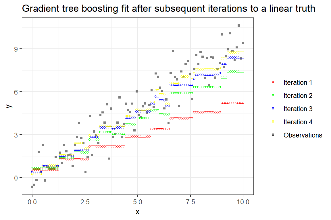
Difficulties with explainability for hundreds or thousands of trees are however a drawback. The following figure illustrates the iterative addition of trees, and eventually obtaining a better fit.
Lazy EDA and feature engineering
Back to the data: Some columns have NA values, however if treated correctly, the algorithm that we will employ is capable of handling this on its own. However, it is necassry to remove uninformative columns: Basic cleaning, uninformative cols
# Uninformative columns
acceptance <- acceptance %>%
    dplyr::select(-c("rank")) %>%
    dplyr::rename(Accepted = "Accepted/unaccepted")

not_informative <- which(acceptance %>% sapply(function(x) length(unique(x))) < 2)
acceptance <- acceptance %>%
    dplyr::select(-c(names(not_informative)))

# Uninformative as direct factor
acceptance[,"Whether taken Before or not"] <- ifelse(is.na(acceptance[,"Whether taken Before or not"]),0,1)

# Character to factor
character_vars <- lapply(acceptance, class) == "character"
acceptance[, character_vars] <- lapply(acceptance[, character_vars], as.factor)
rm(character_vars, not_informative); invisible(gc())
Let’s take a short look at how some variables relate to the response. Lazy EDA
#cbPalette <- c("#000000", "#E69F00", "#56B4E9", "#009E73", "#F0E442", "#0072B2", "#D55E00", "#CC79A7")
cbPalette <- c("#999999", "#E69F00", "#56B4E9", "#009E73", "#F0E442", "#0072B2", "#D55E00", "#CC79A7")

p1 <- acceptance %>%
    ggplot(aes(`total credit of taken courses/total credits for graduation`)) +
    geom_density(aes(alpha=0.5, fill=Accepted)) +
    scale_fill_manual(values=cbPalette) +
    theme_bw()
p2 <- acceptance %>%
    ggplot(aes(x=`applied mileage`)) +
    geom_density(aes(alpha=0.5, fill=Accepted)) +
    scale_fill_manual(values=cbPalette) +
    theme_bw()
p3 <- acceptance %>%
    ggplot(aes(`Prescribed Seats`)) +
    geom_density(aes(alpha=0.5, fill=Accepted)) +
    scale_fill_manual(values=cbPalette) +
    theme_bw()
p4 <- acceptance %>%
    ggplot(aes(x=`Grade (year)`, color=Accepted, fill=Accepted)) +
    geom_histogram(aes(y=..density..), alpha=0.5, position="identity", bins=6) +
    scale_fill_manual(values=cbPalette) +
    theme_bw()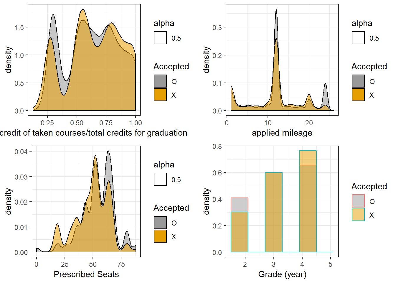
As can be seen, all of these features are somewhat informative (hint, they were not chosen at random).
For feature engineering, I am extremely lazy, and just do the one-hot encoding. This is automatically done by the model.matrix function (which also creates a removable intercept column), with the drawback that NA values are removed. To avoid this, we also employ the model.frame function in the following code:
Creating the model matrix
acceptancemm <- model.matrix(Accepted~.,
                         data= model.frame(Accepted~., data=acceptance, na.action = na.pass))[,-1]
This results in a dataset with quite a lot of columns: the dataset has dimensions 6520, 368.
Finally, we need to split the data in a training and a test set. For this, we use 60% for training and 40% for testing later.
Splitting the data – test and train
set.seed(1432)
train_ind <- sample(nrow(acceptance), 0.6*nrow(acceptance), replace = FALSE)
dtrain <- acceptancemm[train_ind,]
dtest <- acceptancemm[-train_ind,]
y <- ifelse(acceptance$Accepted=="X", 0, 1)
y_train <- y[train_ind]
y_test <- y[-train_ind]
XGBoost parameter tuning
For gradient tree boosting, we employ the amazing XGBoost library. Before we start the training, we need to specify a few hyperparameters. The most important ones are the following
eta: The \(\eta\), typically called the learning rate (the step-length in function space).max_depthA maximum tree depth for all trees.nrounds: The number of boosting iterations.
The following are typically used for regularization.
gamma: Constant penalization for the number of nodes.lambda: L2 regularization.alpha: L1 regularization.
The final ones I’ll mention are the sampling possiblities.
subsample: Row sampling without replacement.colsample_bytree: Column subsampling.
Note that because the row sampling is without replacement, this is not the same type of sampling as the bootstrapping/bagging approach of random forest. See this link for a full parameter specification list.
XGBoost initialization
# Simple model
p.xgb <- list(objective = "binary:logistic",
              booster = "gbtree",
              eval_metric = "logloss",
              nthread = 8,
              eta = 0.3, # no time for low eta
              max_depth = 3,
              min_child_weight =5,
              gamma = 0,
              subsample = 0.8,
              colsample_bytree = 0.6, # ncol(dtrain) is quite large, high sampling
              colsample_bylevel = 0.3,
              alpha = 0, # Tune if time
              lambda = 0,
              nrounds = 1000, # does not matter
              early_stopping_rounds=100)
p.xgb.reg <- p.xgb
We want to specify the hyperparameters in such a way that the model generalizes well to unseen data. To do this, we employ cross validation on a grid of hyperparameters. This is costly, of course, and my grid is therefore not very large. A properly tuned XGBoost model will have to search quite a bit more for optimal tuning.
XGBoost Hyperparemeter search using cross validation
dtrain.xgb <- xgb.DMatrix(data = dtrain, label = y_train)
dtest.xgb <- dtest

gamma.grid <- seq(0,1,length.out=5)
cv.score <- numeric(length(gamma.grid))#matrix(nrow=length(gamma.grid), ncol = length(lambda.grid))
cv.niter <- cv.score
for(j in 1:length(gamma.grid)){
    cat("j iter: ", j, "\n")
    p.xgb.reg$gamma <- gamma.grid[j]
    cv.tmp <- xgb.cv(p.xgb.reg,
                     data = dtrain.xgb, nround = 10000,
                     nfold = 5, prediction = TRUE, showsd = TRUE,
                     early_stopping_round = p.xgb.reg$early_stopping_rounds,
                     maximize = FALSE, verbose = FALSE)
    cv.score[j] <- cv.tmp$evaluation_log[,min(test_logloss_mean)]
    cv.niter[j] <- cv.tmp$best_iteration
}
For this particular search on gamma and nrounds we end up with the values 0.5 and 1436 respectively.
The final model and results
Finally ready for the training phase, this is a one-liner.
Training the final model
mod_xgb <- xgb.train(p.xgb, dtrain.xgb, p.xgb$nrounds)Trees (and ensembles of such) have a natural measure of feature importance. We may use this to see which features are important for the model.
Feature importance
names <- dimnames(dtrain)[[2]]
importance_matrix <- xgb.importance(names, model=mod_xgb)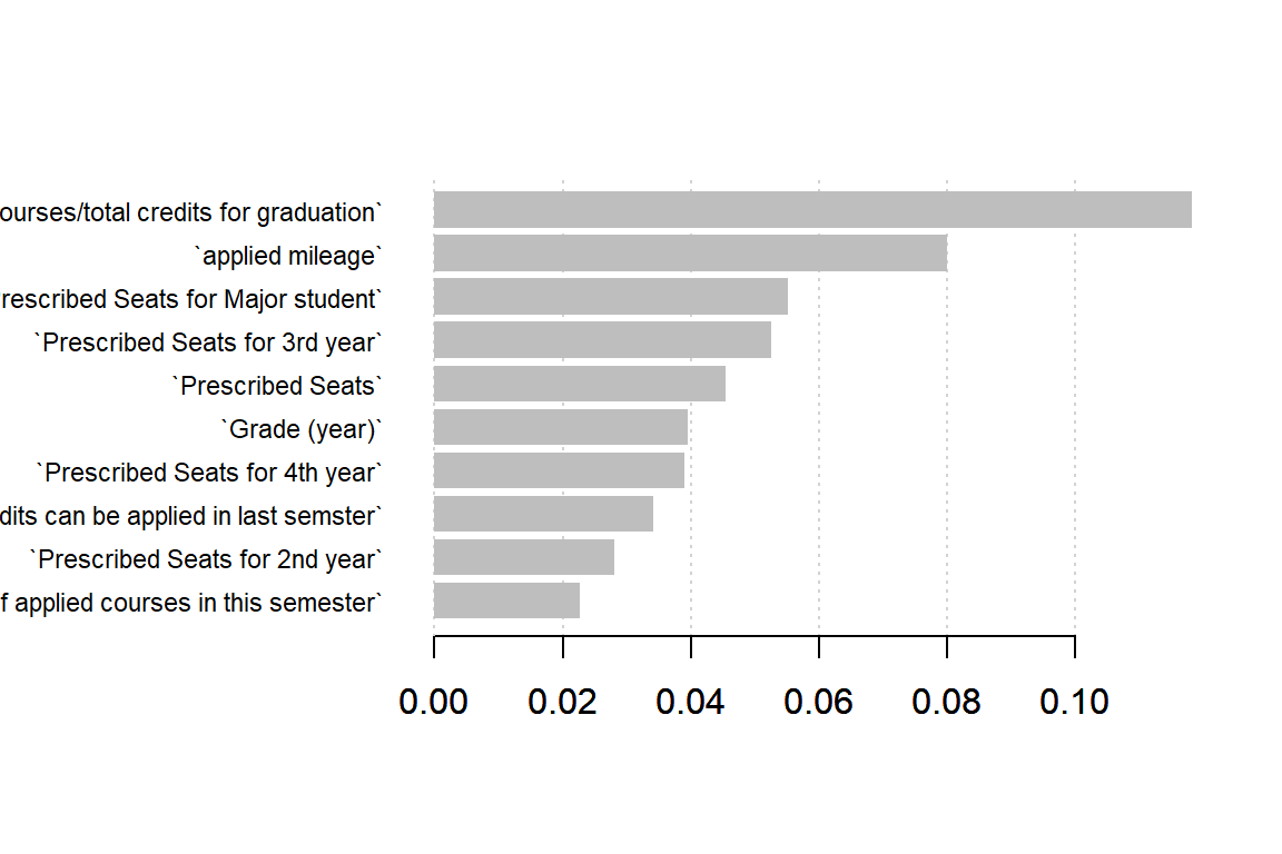
Results
Having trained our model, we wish to see how well it performs on unseen data. Prediction on test
prob.xgb <- xgboost:::predict.xgb.Booster(mod_xgb, dtest)We create a very useful plot for binary classifications: the distribution of the estimated probabilities, conditioned on the outcome, and see if we are able to separate the two classes. In addition, we may check the log-loss values and the accuracy.
Conditional distribution of estimated probabilities
p1 <- data.frame(prob=prob.xgb, Accepted=y_test) %>%
    ggplot(aes(prob)) +
    geom_density(aes(alpha=0.5, fill = factor(Accepted))) +
    xlab("estimated probability") +
    ggtitle("Distribution of estimated probability, conditioned on Accepted") +
    scale_fill_manual(values=cbPalette) +
    theme_bw()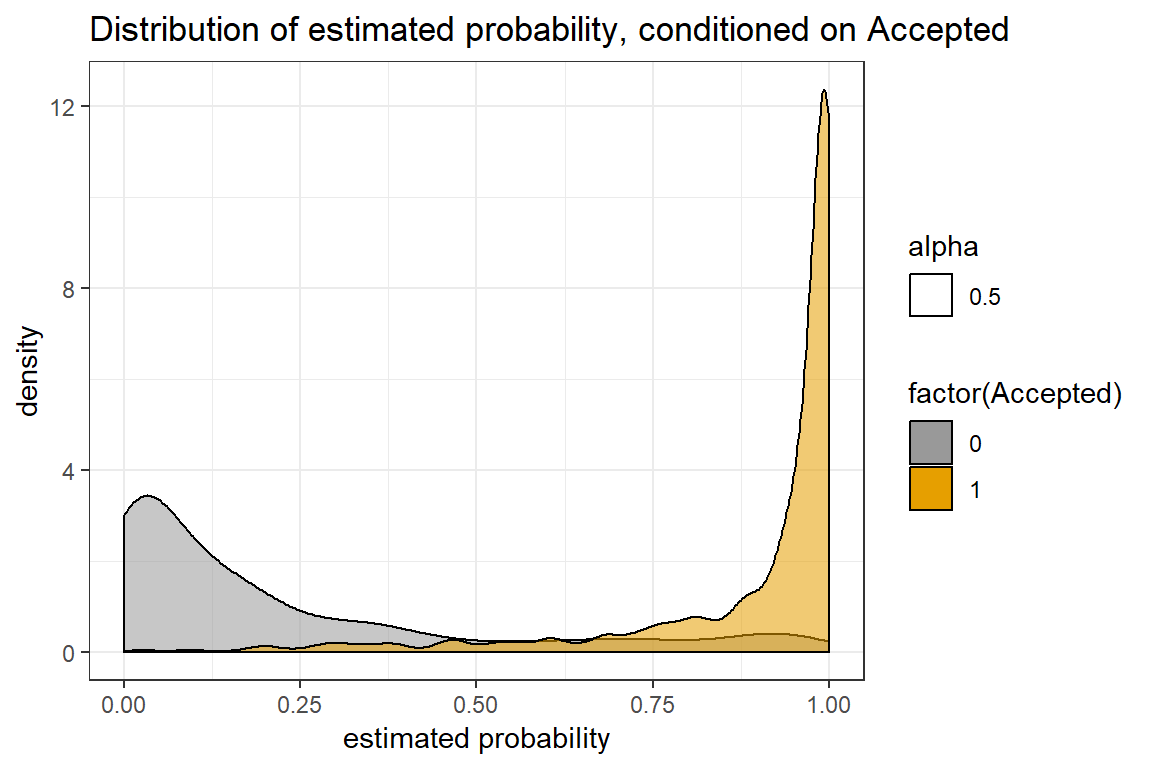
This looks pretty good! Specifically, for the test data, we get a log-loss score at 0.24 and accuracy at 0.91. This is quite good, considering that we did not optimize for accuracy.