We seek to employ the framework of the R package Template Model Builder TMB (Kristensen et al. 2016) which approximately “integrates out” latent variables using the Laplace approximation – to automatically solve the inner problem of the saddlepoint approximation (SPA) and return the negative logarithm of the SPA. All code can be found in this Github repository. The document has the following layout:
- Introduction to the Laplace approximation
- Introduction to the Saddlepoint approximation
- Introduction to TMB
- Using TMB in numerical SPA calculations and parameter optimization
- spaTMB example
Edit 12.04.2019
A TMB fork with SPA functionality installed can be found at this github repository, and installed to R via the command devtools::install_github("Blunde1/adcomp/TMB")
Usage:
- User supplies the objective function f to only be the inner problem of the SPA (renormalization is done automatically).
- Specify the
SPAoption inMakeADFuntoSPA=TRUE(otherwise, the Laplace approximation is calculated). - Specify
random=s(saddlepoints) for TMB to calculate the inner problem.
An example is provided under the name spa_gauss in the examples repository.
I have made a pull-request to the official TMB repository, but this might of course fall through or take some time.
Small change in and before the inverse subset algorithm table: trying to explain a bit more in detail what f and ff corresponds to.
Introduction to the Laplace approximation
We consider the Laplace approximation in the context of likelihood estimation, following (read: stolen from) (Kristensen et al. 2016) completely: Let \(f(\mathbf{u},\theta)\) denote the negative joint log-likelihood of the data and the random effects. This depends on the unknown random effects \(\mathbf{u}\in\mathbb{R}^n\) and parameters \(\theta\in\mathbb{R}^m\). The maximum likelihood estimate for θ maximizes \[ \begin{align*} L(\theta) = \int_{\mathbb{R}^n} \exp(-f(\mathbf{u},\theta)) d\mathbf{u}, \end{align*} \] i.e., the random effects \(\mathbf{u}\) have been integrated out. High-dimensional integration is, in general, difficult, but can be achieved by applying the Laplace approximation, giving the approximation \[ \begin{align*} L^*(\theta) = \frac{\sqrt{2\pi}^n \exp(-f(\mathbf{{\hat{\mathbf{u}}(\theta)}},\theta))}{\sqrt{\| \nabla_\mathbf{u}^2f({\hat{\mathbf{u}}(\theta)},\theta) \|}}, \end{align*} \] where
- \({\hat{\mathbf{u}}(\theta)}= \arg\min_\mathbf{u} f(\mathbf{u},\theta)\),
- and \(\nabla_\mathbf{u}^2f(\mathbf{u},\theta)\) is the Hessian matrix, denoted \(H(\theta)\) from here on out.
Introduction to the Saddlepoint approximation
The SPA takes as a vantage point the following inversion integral: \[ \begin{align*} f_\mathbf{Y}(\mathbf{y};\theta) = \frac{1}{(2\pi)^n} \int_{\mathbb{R}^n} e^{( (\tau + i \mathbf{s})^T \mathbf{y} ) } M_\mathbf{Y}(\tau + i\mathbf{s} ; \theta) d\mathbf{s}. \end{align*} \] where \(i=\sqrt{-1}\), \(M_\mathbf{Y}(\mathbf{s}) = E(\exp(\mathbf{s}^T\mathbf{y}))\) is the moment generating function (MGF), \(\tau\in\mathbb{R}^n\) such that \(E(\exp(\tau^T\mathbf{y})) < \infty\) (Butler 2007).
Applying the Laplace approximation to this integral, we obtain the multivaraite saddlepoint approximation: \[ \texttt{spa}(f;\mathbf{y}) = \frac{\exp\left(K_\mathbf{y}({\hat{\mathbf{s}}(\theta)};\theta)-{\hat{\mathbf{s}}(\theta)}^T \mathbf{y}\right)} {(2\pi)^{(n/2)}\sqrt{\| \nabla_\mathbf{s}^2 K_\mathbf{y}({\hat{\mathbf{s}}(\theta)};\theta) \|}} \]
where
- \(K_\mathbf{y}(\mathbf{s};\theta) = \log M_\mathbf{y}(\mathbf{s};\theta)\),
- \(\nabla_\mathbf{s}^2 K_\mathbf{y}(\mathbf{s};\theta)\) is the Hessian matrix,
- and the saddlepoint \({\hat{\mathbf{s}}(\theta)}\) solves \({\hat{\mathbf{s}}(\theta)}= \arg\min_{\mathbf{s}} K_\mathbf{y}(\mathbf{s};\theta) - \mathbf{s}^T\mathbf{y}\)
see (Kleppe and Skaug 2008) for a very general derivation, or the standard reference (Butler 2007).
Introduction to TMB
Template model builder, or TMB for short, wraps (on the C++ side) the high-performance C++ libraries Eigen (a C++ template library for linear algebra: matrices, vectors, numerical solvers, and related algorithms) and CppAD (templated automatic differentiation using operator overloading), for R users to obtain highly efficient evaluations of objective functions and their derivatives (gradient and Hessian) and with automatically performing the Laplace approximation as its high-point.
The TMB user only has to specify the objective function \(f(\theta)\), or \(f(\mathbf{u}, \theta)\) in the case of latent variables \(\mathbf{u}\) that needs to be integrated out, and TMB takes care of the rest. Specifically, the (negative log) Laplace approximation to the negative joint log-likelihood is returned: \[ - \log L^*(\theta) = -n \log \sqrt{2\pi} + \frac{1}{2}\log \| H(\theta) \| + f({\hat{\mathbf{u}}(\theta)},\theta). \] Using this, the likelihood estimates of \(\theta\), i.e. \(\hat{\theta}=\arg\min_\theta - \log L^*(\theta)\), can be found very efficiently, because TMB also returnes the gradient and (finite difference approximation) Hessian of \(-\log L^*(\theta)\) w.r.t. \(\theta\).
Example from TMB
R code
## Simulate data
set.seed(123)
n <- 10000
sigma <- 0.3
phi <- 0.8
simdata <- function() {
    u <- numeric(n)
    u[1] = rnorm(1)
    if (n >= 2)
        for (i in 2:n) {
            u[i] = phi * u[i - 1] + rnorm(1, sd = sqrt(1 - phi^2))
        }
    u <- u * sigma
    x <- as.numeric(rbinom(n, 1, plogis(u)))
    data <- list(obs = x)
    data
}
##
data <- simdata()
parameters <- list(phi = phi, logSigma = log(sigma))

## Adapt parameter list
parameters$u <- rep(0, n)

require(TMB)
compile("laplace.cpp")
dyn.load(dynlib("laplace"))

obj <- MakeADFun(data, parameters, random = "u", DLL = "laplace")
obj$fn()

system.time(opt <- nlminb(obj$par, obj$fn, obj$gr))
(sdr <- sdreport(obj))
C++ code
#include <TMB.hpp>

template<class Type>
Type objective_function<Type>::operator() ()
{
  DATA_VECTOR(obs);
  PARAMETER(phi);
  PARAMETER(logSigma);
  PARAMETER_VECTOR(u);
  using namespace density;
  Type sigma= exp(logSigma);
  Type f = 0;
  f += SCALE(AR1(phi), sigma)(u);
  vector<Type> p = invlogit(u);
  f -= dbinom(obs, Type(1), p, true).sum();
  return f;
}
Using TMB in numerical SPA calculations and parameter optimization
Set the goal of making TMB automatically solve the inner problem of the SPA, and returning the negative log SPA for the purpose of likelihood optimisation. Ideally, we would have TMB return \[
-\log \texttt{spa}(f,\mathbf{y})
= \frac{1}{2}\left( \log \| \nabla_\mathbf{s}^2 K_\mathbf{y}({\hat{\mathbf{s}}(\theta)};\theta) \| + n\log(2\pi) \right) -
\left(K_\mathbf{y}({\hat{\mathbf{s}}(\theta)};\theta)-{\hat{\mathbf{s}}(\theta)}^T \mathbf{y}\right).
\] However, to solve the inner problem of the SPA, we need to supply the following objective: \[
\begin{align*}
f(\mathbf{u},\theta) &= K_\mathbf{y}(\mathbf{s};\theta) - \mathbf{s}^T\mathbf{y} - n\log (2\pi)\\
&\approx K_\mathbf{y}(\mathbf{s};\theta) - \mathbf{s}^T\mathbf{y},
\end{align*}
\] where \(\mathbf{s}\) is set to random (and hence, will be integrated out by TMB). However, TMB would then return \[
- \log L^*(\theta) = -\log \texttt{spa}(f,\mathbf{y}) + 2 \left(K_\mathbf{y}({\hat{\mathbf{s}}(\theta)};\theta)-{\hat{\mathbf{s}}(\theta)}^T \mathbf{y}\right).
\] i.e., the sign is reversed on \(f(\mathbf{u},\theta) \sim K_\mathbf{y}({\hat{\mathbf{s}}(\theta)};\theta)-{\hat{\mathbf{s}}(\theta)}^T \mathbf{y}\). This is because, for the SPA, the Laplace approximation is calculated w.r.t. the objective \[
f(\mathbf{u},\theta) = K_\mathbf{y}(\mathbf{\tau} + i\mathbf{s};\theta) - (\mathbf{\tau} + i\mathbf{s})^T\mathbf{y} - n\log (2\pi),
\] where the imaginary unit, \(i\), reverses the sign of the Hessian (w.r.t \(\mathbf{\tau}\)), replacing minimization with maximization in the the inner optimization and vice versa. TMB does not directly allow complex AD data types (while still possible inside TMB, see e.g. this file on Github and example use (advanced SPA calculations) in corresponding repository).
There are at least four possible solutions:
- Use the
autodiffnamespace to construct structs of \(K\) and the inner problem, and a Newton type algorithm to solve it. This is not ideal, because all Newton iterations will be taped by TMB, while only the last two should be sufficient for derivatives w.r.t. \(\theta\). See this code for an example. - Use
ADREPORTon the quantities needed to build the negative \(\log \texttt{spa}\) and its gradient - Use the quantities in
obj$envto build newobj$fnandobj$gr. - Update
MakeADFunwith aspa=TRUEoption, such that SPA calculations are performed instead of Laplace. This would essentially do the same as point three (but be under the hood).
I have done a hybrid between point 3 and 4; ideally I would like to make a branch on my TMB installation to do point 4, but I am on a Windows machine and hence not blessed with the developer version. If this works, I will still make a pull-request (however, untried) on MakeADFun with a SPA option to adcomp/TMB.
To update MakeADFun or obj$env, the source code must be studied. The TMB user will be familiar with obj$fn(), obj$gr() and perhaps obj$he(), which, if random is unspecified, correspond to the user supplied objective function, its gradient and Hessian. In this case, this correspond to the function f of orders \(0:2\) inside of MakeADFun which it will eventually return when random is unspecified. Otherwise, obj$fn() and obj$gr() will correspond to the Laplace approximation of the user supplied objective function and its gradient. In this case the function ff is calculated internally of MakeADFun and eventually returned. The following table summarizes my findings (conditioned on no special options evoked in the MakeADFun call). Here, we write \(l\) for the Laplace approximation and \(h\) for the functional form (but unsolved inner problem), denote partial derivatives by subscripts, i.e. \(H=f_{\mathbf{u}\mathbf{u}}\), and write \(\mathbf{\nu}=(\mathbf{u},\theta)\) for the collection of parameters.
| Name | Order | Mathemtical expression | Description |
|---|---|---|---|
f |
order==0 |
\(f(\mathbf{u},\theta)\) | The user supplied objective |
order==1 |
\(f_\mathbf{\nu}(\mathbf{u},\theta)\) | The gradient of user objective | |
order==2 |
\(f_{\mathbf{\nu} \mathbf{\nu}}(\mathbf{u},\theta)\) | The Hessian matrix of \(f\) w.r.t. all parameters | |
h |
order==0 |
\(h(\mathbf{u},\theta)=f(\mathbf{u},\theta) + \frac{1}{2}\log\| f_{\mathbf{u}\mathbf{u}}(\mathbf{u},\theta) \| - \frac{n}{2}\log(2\pi)\) | The Laplace objective |
order==1 |
\(h_\nu(\mathbf{u},\theta)=f_\mathbf{\nu}(\mathbf{u},\theta) + \frac{1}{2}\nabla_\nu \log\|f_{\mathbf{u}\mathbf{u}}(u,\theta) \|\) | The derivative of the Laplace objective w.r.t. all parameters | |
ff |
order==0 |
\(l(\theta)=h({\hat{\mathbf{u}}(\theta)},\theta);~ {\hat{\mathbf{u}}(\theta)}=\arg\min_\mathbf{u} f(\mathbf{u},\theta)\) | h(order=0) at \(\mathbf{u}={\hat{\mathbf{u}}(\theta)}\) |
order==1 |
\(\begin{align}l_\theta(\theta) &= h_\theta({\hat{\mathbf{u}}(\theta)},\theta)\\ &-h_\mathbf{u}({\hat{\mathbf{u}}(\theta)},\theta)f_{\mathbf{u}\mathbf{u}}({\hat{\mathbf{u}}(\theta)},\theta)^{-1} f_{\mathbf{u}\theta}({\hat{\mathbf{u}}(\theta)},\theta)\end{align}\) | Gradient of the Laplace approximation w.r.t. \(\theta\) |
A side note
The expression \(\nabla_\nu \log\|f_{\mathbf{u}\mathbf{u}}(u,\theta) \|\) in $h(order==1) is difficult and deserve special attention. From (Searle, Casella, and McCulloch 2009) page 457 or (Kristensen et al. 2016) eq.8, we have for an individual element \(\nu_j\)
\[ \frac{\partial}{\partial \nu_j} \log\|f_{\mathbf{u}\mathbf{u}}(u,\theta) \| = \mathrm{tr}\left( f_{\mathbf{u}\mathbf{u}}(u,\theta)^{-1} \frac{\partial}{\partial \nu_j} f_{\mathbf{u}\mathbf{u}}(u,\theta) \right). \] This can also be solved purely by using AD, see Table 1 in (Skaug and Fournier 2006).
From this summary, it should be clear that if we
- Supply the objective function \[f(\mathbf{u},\theta) = K_\mathbf{y}(\mathbf{s};\theta) - \mathbf{s}^T\mathbf{y} - n\log (2\pi)\] With \(\mathbf{s}\) set to
random. - Manipulate
h(order=0)to return the negative log SPA \[h(\mathbf{u},\theta)= -f(\mathbf{u},\theta) + \frac{1}{2}\log\| f_{\mathbf{u}\mathbf{u}}(\mathbf{u},\theta) \| - \frac{n}{2}\log(2\pi)\]. - Manipulate
h(order=1)to the negative log spa derivative: \[ \begin{align} h_\nu(\mathbf{u},\theta)= - f_\mathbf{\nu}(\mathbf{u},\theta) + \frac{1}{2}\nabla_\nu \log\|f_{\mathbf{u}\mathbf{u}}(u,\theta) \| \end{align} \]
then TMB will take care of the rest. The R code for the “fix” is provided below.
R code for solution
# after MakeADFun
library(Matrix)
attach(obj$env)
# update h
obj$env$h <- function(theta = par, order = 0, hessian, L, ...) {
    if (order == 0) {
        ## logdetH <- determinant(hessian)$mod
        logdetH <- 2 * determinant(L)$mod
        ans <- -f(theta, order = 0) + 0.5 * logdetH - length(random)/2 * log(2 *
            pi)  #### updated
        if (LaplaceNonZeroGradient) {
            grad <- f(theta, order = 1)[random]
            ans - 0.5 * sum(grad * as.numeric(solveCholesky(L, grad)))
        } else ans
    } else if (order == 1)
        {
            if (LaplaceNonZeroGradient)
                stop("Not correct for LaplaceNonZeroGradient=TRUE")
            ## browser()
            e <- environment(spHess)
            solveSubset <- function(L) .Call("tmb_invQ", L, PACKAGE = "TMB")
            solveSubset2 <- function(L) .Call("tmb_invQ_tril_halfdiag", L, PACKAGE = "TMB")
            ## FIXME: The following two lines are not efficient: 1. ihessian <-
            ## tril(solveSubset(L)) 2. diag(ihessian) <- .5*diag(ihessian) Make option to
            ## solveSubset to return lower triangular part with diagonal halved. As it is
            ## now the output of solveSubset is symm _with upper storage_ (!) (side
            ## effect of cholmod_ptranspose) therefore tril takes long time. Further,
            ## 'diag<-' is too slow.  FIXED! :
            ihessian <- solveSubset2(L)
            ## Profile case correction (1st order case only)
            if (!is.null(profile)) {
                ## Naive way: ihessian[profile,] <- 0 ihessian[,profile] <- 0 However, this
                ## would modify sparseness pattern and also not account for 'ihessian' being
                ## permuted:
                perm <- L@perm + 1L
                ihessian <- .Call("tmb_sparse_izamd", ihessian, profile[perm],
                  0, PACKAGE = "TMB")
            }

            ## General function to lookup entries A subset B.  lookup.old <-
            ## function(A,B){ A <- as(tril(A),'dtTMatrix') B <- as(tril(B),'dtTMatrix')
            ## match(paste(A@i,A@j),paste(B@i,B@j)) } General function to lookup entries
            ## A in B[r,r] assuming pattern of A is subset of pattern of B[r,r].
            lookup <- function(A, B, r = NULL) {
                A <- tril(A)
                B <- tril(B)
                B@x[] <- seq.int(length.out = length(B@x))  ## Pointers to full B matrix (Can have up to 2^31-1 non-zeros)
                if (!is.null(r)) {
                  ## Goal is to get: B <- forceSymmetric(B) B <- B[r,r,drop=FALSE] However the
                  ## internal Matrix code for 'B[r,r,drop=FALSE]' creates temporary 'dgCMatrix'
                  ## thereby almost doubling the number of non-zeros. Need solution that works
                  ## with max (2^31-1) non-zeros:
                  B <- .Call("tmb_half_diag", B, PACKAGE = "TMB")
                  B <- tril(B[r, r, drop = FALSE]) + tril(t(B)[r, r, drop = FALSE])
                }
                m <- .Call("match_pattern", A, B, PACKAGE = "TMB")  ## Same length as A@x with pointers to B@x
                B@x[m]
            }
            if (is.null(e$ind1)) {
                ## hessian: Hessian of random effect part only.  ihessian: Inverse subset of
                ## hessian (same dim but larger pattern!).  Hfull: Pattern of full hessian
                ## including fixed effects.
                if (!silent)
                  cat("Matching hessian patterns... ")
                iperm <- invPerm(L@perm + 1L)
                e$ind1 <- lookup(hessian, ihessian, iperm)  ## Same dimensions
                e$ind2 <- lookup(hessian, e$Hfull, random)  ## Note: dim(Hfull)>dim(hessian) !
                if (!silent)
                  cat("Done\n")
            }
            w <- rep(0, length = length(e$Hfull@x))
            w[e$ind2] <- ihessian@x[e$ind1]
            ## Reverse mode evaluate ptr in rangedirection w now gives .5*tr(Hdot*Hinv)
            ## !!  return
            as.vector(-f(theta, order = 1)) + .Call("EvalADFunObject", e$ADHess$ptr,
                theta, control = list(order = as.integer(1), hessiancols = as.integer(0),
                  hessianrows = as.integer(0), sparsitypattern = as.integer(0),
                  rangecomponent = as.integer(1), rangeweight = as.double(w),
                  dumpstack = as.integer(0), doforward = as.integer(1)), PACKAGE = DLL)
        }  ## order == 1
 else stop(sprintf("'order'=%d not yet implemented", order))
}  ## end{ h }
spaTMB example
Finally, an example for which we know the true solution is supplied: The Gaussian case.
First, we need to specify the objective function. That is, of course, the inner problem with a normalizing constant:
#include <TMB.hpp>

template<class Type>
Type objective_function<Type>::operator() ()
{
    DATA_VECTOR(y);
    PARAMETER(mu);
    PARAMETER(logSigma);
    PARAMETER_VECTOR(s); // saddlepoints

    // Return K_y(s)-s^T y - n/2 log(2*pi)
    // K_y(s) = sum K_{y[i]}(s[i])
    // K_N(mu, logSigma)(s) = mu*s + sigma^2 * s^2 / 2

    Type sigma = exp(logSigma);
    int n = y.size();

    // Build CGF
    Type K = 0;
    for(int i=0; i<n; i++){
        K += mu * s(i) + 0.5*s(i)*s(i)*sigma*sigma;
    }

    // Build inner problem with normalization constant
    Type res = K - (s*y).sum() - n * log(2*M_PI);

    // report sigma
    ADREPORT(sigma);

    return res;
}
On the R side, we do what is described in the previous section:
# Simulate data
set.seed(123)
n <- 10000
mu <- 3
sigma <- 1.5
y <- rnorm(n, mu, sigma)

# data and parameters
data <- list(y=y)
parameters <- list(mu=0, logSigma = log(1), s=numeric(n))

# Compile c++ code and load into R
library(TMB)
compile("gauss_spa_example.cpp")
[1] 0
dyn.load(dynlib("gauss_spa_example"))

# create adfun, set s="random" for SPA inner problem
obj <- MakeADFun(data, parameters, random="s", DLL="gauss_spa_example", silent = T)

# update obj$env$e functions to calculate SPA
source("spaTMB.R")

# optimize
opt <- nlminb(obj$par, obj$fn, obj$gr)
rep <- sdreport(obj)
knitr::kable(rbind(summary(rep, "fixed", p.value = TRUE),
                   summary(rep, "report", p.value = TRUE))) %>%
kable_styling(full_width = F)| Estimate | Std. Error | z value | Pr(>|z^2|) | |
|---|---|---|---|---|
| mu | 2.9964425 | 0.0149788 | 200.04556 | 0 |
| logSigma | 0.4040508 | 0.0070711 | 57.14143 | 0 |
| sigma | 1.4978800 | 0.0105916 | 141.42141 | 0 |
The likelihood estimates are on point!
We should also check that the value of the negative log SPA matches that of the negative log normal density for the observations (this is very likely, hinging on the successful parameter optimisation), since the SPA is exact in the normal case. Also, if the gradient is zero at the optimum, we can be relatively safe that everything is okay.
obj$fn(opt$par)## [1] 18229.89
## attr(,"logarithm")
## [1] TRUE-sum(dnorm(y, opt$par[1], exp(opt$par[2]), log=TRUE))## [1] 18229.89obj$gr(opt$par)## [1] 0.0002041866 -0.0002949115The negative log SPA and its gradient are implemented correctly!!
Note that TMB is extremely fast, and even with 10000 “latent” variables (read: saddlepoints), the computations are done within a second on my computer. Finally, for the Gaussian case, we may calculate the saddlepoints explicitly to check that everything matches: \[ \begin{align} {\hat{\mathbf{s}}(\theta)}&= \arg\min_s (K_Y(s)-sy) \\ {\hat{\mathbf{s}}(\theta)}&: K_Y'(s) -x = 0\\ K_Y(s) &= \mu s + \frac{1}{2}s^2\sigma^2 \text{ in the Gaussian case, thus }\\ {\hat{\mathbf{s}}(\theta)}&= \frac{x-\mu}{\sigma^2} \end{align} \]
# check s = normal sp and parameters
plot(summary(rep, "random")[,"Estimate"], (y-opt$par[1])/(exp(opt$par[2]))^2,
main="Numerical versus theoretical saddlepoints",
xlab="Numerical", ylab="Theoretical")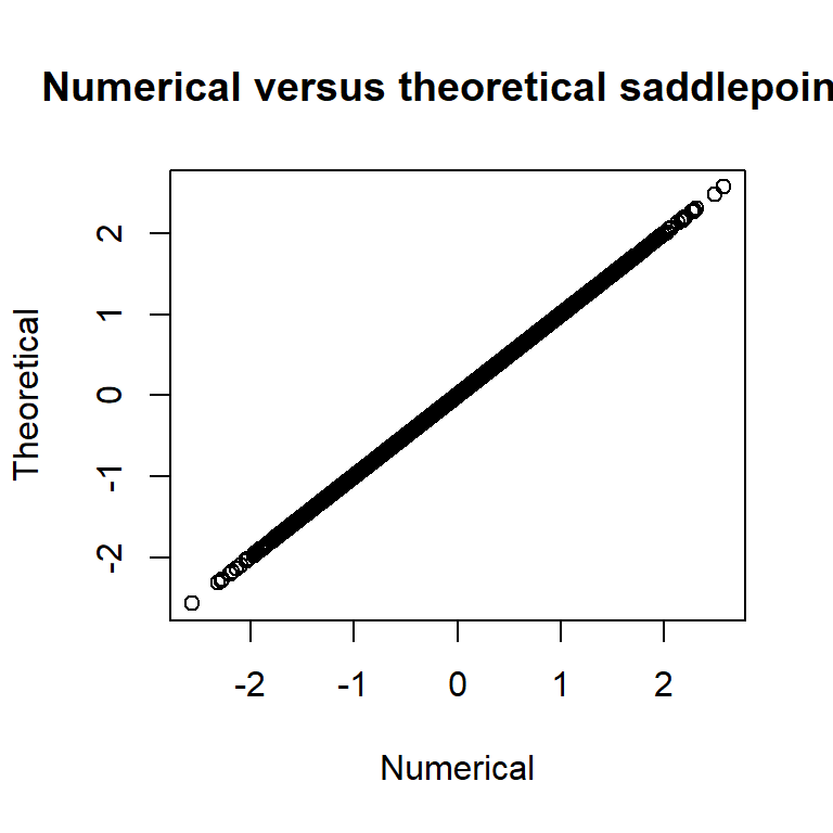 and we see that the numerical quantities matches the theoretical ones.
This is pretty cool! We now only need to supply the inner problem of the SPA (typically very little code) and a normalization constant, and TMB will take care of everything in the fastest possible way! I will proceed to make a pull request soon.
Butler, Ronald W. 2007. Saddlepoint Approximations with Applications. Cambridge University Press.
Kleppe, Tore Selland, and Hans J Skaug. 2008. “Building and Fitting Non-Gaussian Latent Variable Models via the Moment-Generating Function.” Scandinavian Journal of Statistics 35 (4). Wiley Online Library: 664–76.
Kristensen, Kasper, Anders Nielsen, Casper W Berg, Hans Skaug, and Bradley M Bell. 2016. “TMB: Automatic Differentiation and Laplace Approximation.” Journal of Statistical Software 70 (i05). Foundation for Open Access Statistics.
Searle, Shayle R, George Casella, and Charles E McCulloch. 2009. Variance Components. Vol. 391. John Wiley & Sons.
Skaug, Hans J, and David A Fournier. 2006. “Automatic Approximation of the Marginal Likelihood in Non-Gaussian Hierarchical Models.” Computational Statistics & Data Analysis 51 (2). Elsevier: 699–709.