In my previous post, I mentioned my friend and previous co-worker at Tryg, Ole Schei, that is wonderfully meticulous, and has for some time quantified aspects of his life in a time-series format. This is, of course, a natural thing to do for an actuary. While we both worked at Tryg I was allowed to look at one of these time-series – the one containing detailed information about Ole’s web-surfing (for non work-related matters) at work. This has since become my favourite dataset, perhaps because of the way it was created, but also because the modelling is fun and the absurdity in modelling Ole as a mean-reverting doubly stochastic Poisson process (which we will eventually do). I will here work on an aggregated version of these data. As usual, click the arrows to see the code.
These data are visualized in the next figure. In this plot, I’ve added a constant line, which refers to the expected number web-surfs per day, given that Ole is a Poisson process with constant intensity.
Ole as an ordinary Poisson process
# Build the likelihood function
jnll <- function(lambda){
    -sum(dpois(N,lambda*7,log=TRUE))
}

# Optimize the likelihood
opt_pois <- nlminb(1,jnll,lower=0)

# Throw data into a data frame
data <- data.frame("daily_surfs"=N,
                   "time"=1:length(N),
                   "constant_intensity"=rep(opt_pois$par*7, length(N)))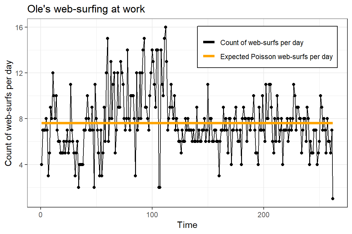
It is easy to see that Ole is no ordinary constant-intensity Poisson process. He is a complex being, and cannot be reducted to such a simple object! A doubly stochastic Poisson process is much more appropriate. For such a model the intensity for which he surfs is much more flexible (and stochastic). To truly understand him (and his surf-intensity/urge-to-surf), we must ask ourselves: what is Ole?
Answers
- Ole lives in continuous-time.
- Ole’s underlying urge to surf the web is what governs his realizations.
- Random events influence his mood and urge to surf from time to time.
- Ole is not a slave, he has some free will and the power to express it. His urge for web-surfing therefore never goes to zero.
- He is neither an addict, nor does he hate his work (to the best of my knowledge). The counts of web-surfs therefore does not sky-rocket.
These properties suggest a continous-time process that is strictly positive, has a mean-reverting property and therefore stops the web-surfing from taking off. One such model is the Cox-Ingersoll-Ross (CIR) model, defined by the stochastic differential equation (SDE) \[d\lambda_t = \kappa (\alpha - \lambda_t)dt + \sigma \sqrt(\lambda_t) dW_t.\]
Let the urge to surf, integrated over a day, \(u_t=\int_{t_0}^t \lambda_s ds\) be given, then the probability mass function is given as \[p(n) =\frac{u_t^n e^{-u}}{n!}.\]
Our problem is that \(u_t\) is unobserved. My original idea was to use that \(\lambda_t\) is of the affine type, and therefore the characteristic function of \(u_t\) is easily given as \[\varphi_{u_t}(s) = \int_{\Omega} e^{isu_t}p(u_t) du_t = e^{A(t_0,t) + B(t_0,t)\lambda_{t_0}},\] where \(A\) and \(B\) are found from solving a system of Ricatti differential equations. Inverting the characteristic function to obtain the density, we may build the joint likelihood for observed number of surf-times and integrated intensities, and finally integrate out everything that is latent. I implemented this, but have been struggelig with some numerical issues. I will try to work out the numerics later, but for this post, we do an approximation to \(u_t\) and the distribution of \(\lambda_t\) that turns out to work okay.
First, do an Euler approximation on the dynamics of Ole’s urge: \[\lambda_t \approx \lambda_{t_0} + \kappa (\alpha - \lambda_{t_0})dt + \sigma \sqrt(\lambda_{t_0}) N\left(0,\sqrt(dt)\right)\] which is obviously normally distributed. Next, use some numerical scheme to integrate to \(u\). Here, I’ll just use the elementary trapezoid rule: \(u_t = dt (\lambda_t - \lambda_{t_0})/2\), in which \(dt=7\) for a typical work-day for Ole. In this setup, the only thing latent is \(\{\lambda_i\}_{i=1}^n\) corresponding to the time-points of the observations. Finally, I will use the Laplace approximation to integrate out the latent variables. TMB is used for calculations.
TMB infill approximate COX
// Likelihood density of a doubly stochastic Poisson process

#include<TMB.hpp>

template<class Type>
Type trapezoid_rule(Type fa, Type fb, Type dt){
    return dt* (fb+fa)/2;
}


template<class Type>
Type objective_function<Type>::operator()()
{
    DATA_VECTOR(N);
    DATA_SCALAR(dt); // timestep between lambdas
    //DATA_INTEGER(ghiter);
    PARAMETER(kappa);
    PARAMETER(alpha);
    PARAMETER(logSigma); Type sigma = exp(logSigma);
    PARAMETER_VECTOR(logLambda); matrix<Type> lambda = exp(logLambda.array()); // (n+1 X m)
    //PARAMETER_MATRIX(logLambda);
    //vector<Type> lambda = log.Lambda.exp();

    Type nll = 0;
    Type drift, diffusion;
    int n = N.size(); // Number of observations
    int m = lambda.cols(); // Number of infill random effects
    int i=0, j=0; // Iterators

    // CIR: dX = kappa*(alpha-X)dt + sigma*sqrt(X)dW

    /** Contribution from infill intensity random effect */
    Type log_c, q, omega, log_u, log_v;
    log_c = log(2*kappa) - log(1-exp(-kappa*dt)) - 2*log(sigma); // 24: 24 hours
    q = 2*kappa*alpha / (sigma*sigma);

    // first observation - asymptotic distribution
    omega = 2*kappa/(sigma*sigma);
    nll -= q*log(omega) + (q-1)*log(lambda(0,0)) - omega*lambda(0,0) - lgamma(q);
    for(j=1; j<m; j++){
        // Intensities conditioned on previous intensities same day
        drift = lambda(i,j-1) + kappa*(alpha - lambda(i, j-1))*dt;
        diffusion = sigma * sqrt(lambda(i, j-1)*dt);
        nll -= dnorm(lambda(i,j), drift, diffusion, true);
    }

    // All other random effects
    for(i=1; i<(n+1); i++){
        // First intensity current day conditioned on last intensity previous day
        drift = lambda(i-1,m-1) + kappa*(alpha - lambda(i-1, m-1))*dt;
        diffusion = sigma * sqrt(lambda(i-1, m-1)*dt);
        nll -= dnorm(lambda(i,0), drift, diffusion, true);
        for(j=1; j<m; j++){
            // Intensities conditioned on previous intensities same day
            drift = lambda(i,j-1) + kappa*(alpha - lambda(i, j-1))*dt;
            diffusion = sigma * sqrt(lambda(i, j-1)*dt);
            nll -= dnorm(lambda(i,j), drift, diffusion, true);
            }
    }

    /** Contribution from observations */
    //vector<Type> u = lambda.rowwise().sum() * dt; // Box integration
    vector<Type> u(n); // Trapezoid rule
    u.setZero();
    for(i=0; i<n; i++){
        u(i) += lambda(i,0);
        for(j=1; j<m; j++){
            u(i) += 2*lambda(i,j);
        }
        u(i) += lambda(i+1,0);
        u(i) = dt * u(i) / 2;
    }
    ADREPORT(u);
    for(i=0; i<n; i++){
        nll -= (N[i]*log(u[i]) - u[i] - lgamma(N[i]+1));
    }

    return nll;

}
Correspoding R code for optimization
compile("surfing-the-web-at-work/mrdspp_euler.cpp")## [1] 0dyn.load(dynlib("surfing-the-web-at-work/mrdspp_euler"))
#control
N <- N
kappa <- 0.2
alpha <- 2
sigma <- 0.1
m <- 1
dt <- 7 / m # 7 hour work day divided by m
lambda <- matrix(alpha, nrow=length(N)+1, ncol=m)
DATA <- list(N=N, dt=dt)
PARAMETERS <- list(kappa=kappa, alpha=alpha, logSigma=log(sigma), logLambda=log(lambda))
obj <- MakeADFun( DATA, PARAMETERS, random=c("logLambda"), silent = T )
opt <- nlminb(obj$par, obj$fn, obj$gr)
rep <- sdreport(obj)Did we converge? TRUE.
Finally, we plot the results.
Organizing TMB results and plotting
# Information from report, fixed effects
srep_fixed <- summary(rep, select = c("report", "fixed"), p.value = TRUE) %>%
    tibble::as_tibble(rownames = NA) %>%
    tibble::rownames_to_column() %>%
    dplyr::rename(parameter = rowname,
                  estimate = Estimate,
                  std_error = `Std. Error`,
                  z_value = `z value`,
                  p_value = `Pr(>|z^2|)`) %>%
    mutate(type = "fixed")

# Information from report, random effects
srep_random <- summary(rep, select = c("random"), p.value = TRUE) %>%
    tibble::as_tibble(rownames = NA) %>%
    tibble::rownames_to_column() %>%
    dplyr::rename(parameter = rowname,
                  estimate = Estimate,
                  std_error = `Std. Error`,
                  z_value = `z value`,
                  p_value = `Pr(>|z^2|)`) %>%
    mutate(type = "random") %>%
    dplyr::mutate(parameter = ifelse(parameter == "h", paste0("h", 1:n()), parameter))

# Combine information
srep <- dplyr::bind_rows(srep_fixed, srep_random)

# Add data information and confidence estimates
report <- srep %>%
    filter(parameter == "u") %>%
    mutate(
        N = N,
        time = 1:n(),
        Poisson = opt_pois$par * dt,
        lt_int_mean = opt$par["alpha"]*dt,
       u_upper = estimate + 2 * std_error,
       u_lower = estimate - 2 * std_error,
       N_upper = estimate + 2*sqrt(estimate),
       N_lower = estimate - 2*sqrt(estimate))

# Colours for plot
cols <- c("Estimated stochastic intensity"="black",
          "Realizations of Ole"="lightgrey",
          "Intensity 95% Confidence Interval"="red",
          "Constant Poisson intensity" = "orange",
          "Asymptotic integrated intensity" = "blue",
          "Process 95% Confidence Interval" = "lightblue")
p <-
    ggplot(report) +
    geom_line(aes(time, estimate, color="Estimated stochastic intensity"), size = 2) +
    geom_line(aes(time, N, color="Realizations of Ole")) +
    geom_point(aes(time, N), shape=15, color="black", size=1, alpha=0.5) +
    geom_line(aes(time, u_upper, color="Intensity 95% Confidence Interval"),size = 0.3) +
    geom_line(aes(time, u_lower, color="Intensity 95% Confidence Interval"), size = 0.3) +
    geom_ribbon(aes(time, ymax = u_upper, ymin = u_lower), fill = "red", alpha= 0.10) +
    geom_line(aes(time, Poisson, color="Constant Poisson intensity"), size=1.5, linetype="dashed") +
    geom_line(aes(time, lt_int_mean, color="Asymptotic integrated intensity"), size=1.5, linetype="dashed") +
    geom_line(aes(time, N_upper, color="Process 95% Confidence Interval"), size=0.3) +
    geom_line(aes(time, N_lower, color="Process 95% Confidence Interval"), size=0.3) +
    geom_ribbon(aes(time, ymax = N_upper, ymin = N_lower), fill = "blue", alpha= 0.02) +
    ggtitle("Ole's web-surfing at work: A mean-reverting doubly stochastic Poisson process") +
    xlab("Day") +
    ylab("Count of surfs per day") +
    scale_color_manual(name=NULL, values=cols) +
    scale_linetype_manual() +
    #theme(legend.position=c(.80, .85),legend.background=element_rect(colour='black')) +
    theme_bw()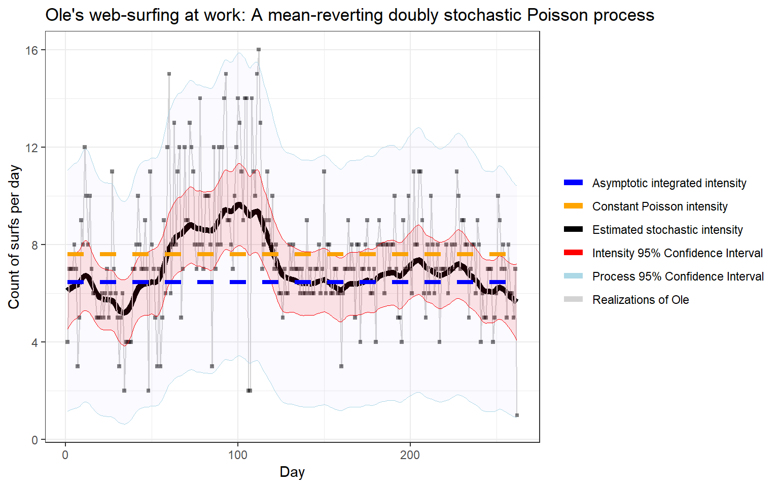
Here is quite a bit of information: The data and constant Poisson intensity from before is in the background. In addition the constant line from the asymptotic integrated intensity (blue, constant) is also plotted. More interestingly, the thick black line is the MAP estimate of the integrated intensity \(u_t\), which has a 95% confidence band (red) around it. Using this, we can also create a confidence band about the actual observations \(\{N_i\}_{i=1}^T\) (light-grey). This nicely wraps the observations. Ole is indeed a complex object!
I will try to work out the numerics for using the Affine properties of the CIR, together with the implementation of exact numeric derivatives of the Bessel function (using Tiny_ad) in TMB.